9. Job Search#
GPU
This lecture was built using a machine with JAX installed and access to a GPU.
To run this lecture on Google Colab, click on the “play” icon top right, select Colab, and set the runtime environment to include a GPU.
To run this lecture on your own machine, you need to install Google JAX.
In this lecture we study a basic infinite-horizon job search with Markov wage draws
The exercise at the end asks you to add recursive preferences and compare the result.
In addition to what’s in Anaconda, this lecture will need the following libraries:
!pip install quantecon
Show code cell output
Requirement already satisfied: quantecon in /opt/conda/envs/quantecon/lib/python3.11/site-packages (0.7.2)
Requirement already satisfied: numba>=0.49.0 in /opt/conda/envs/quantecon/lib/python3.11/site-packages (from quantecon) (0.59.0)
Requirement already satisfied: numpy>=1.17.0 in /opt/conda/envs/quantecon/lib/python3.11/site-packages (from quantecon) (1.26.4)
Requirement already satisfied: requests in /opt/conda/envs/quantecon/lib/python3.11/site-packages (from quantecon) (2.31.0)
Requirement already satisfied: scipy>=1.5.0 in /opt/conda/envs/quantecon/lib/python3.11/site-packages (from quantecon) (1.11.4)
Requirement already satisfied: sympy in /opt/conda/envs/quantecon/lib/python3.11/site-packages (from quantecon) (1.12)
Requirement already satisfied: llvmlite<0.43,>=0.42.0dev0 in /opt/conda/envs/quantecon/lib/python3.11/site-packages (from numba>=0.49.0->quantecon) (0.42.0)
Requirement already satisfied: charset-normalizer<4,>=2 in /opt/conda/envs/quantecon/lib/python3.11/site-packages (from requests->quantecon) (2.0.4)
Requirement already satisfied: idna<4,>=2.5 in /opt/conda/envs/quantecon/lib/python3.11/site-packages (from requests->quantecon) (3.4)
Requirement already satisfied: urllib3<3,>=1.21.1 in /opt/conda/envs/quantecon/lib/python3.11/site-packages (from requests->quantecon) (2.0.7)
Requirement already satisfied: certifi>=2017.4.17 in /opt/conda/envs/quantecon/lib/python3.11/site-packages (from requests->quantecon) (2024.2.2)
Requirement already satisfied: mpmath>=0.19 in /opt/conda/envs/quantecon/lib/python3.11/site-packages (from sympy->quantecon) (1.3.0)
WARNING: Running pip as the 'root' user can result in broken permissions and conflicting behaviour with the system package manager. It is recommended to use a virtual environment instead: https://pip.pypa.io/warnings/venv
We use the following imports.
import matplotlib.pyplot as plt
import quantecon as qe
import jax
import jax.numpy as jnp
from collections import namedtuple

jax.config.update("jax_enable_x64", True)
9.1. Model#
We study an elementary model where
jobs are permanent
unemployed workers receive current compensation \(c\)
the wage offer distribution \(\{W_t\}\) is Markovian
the horizon is infinite
an unemployment agent discounts the future via discount factor \(\beta \in (0,1)\)
The wage process obeys
We discretize this using Tauchen’s method to produce a stochastic matrix \(P\)
Since jobs are permanent, the return to accepting wage offer \(w\) today is
The Bellman equation is
We solve this model using value function iteration.
Let’s set up a namedtuple to store information needed to solve the model.
Model = namedtuple('Model', ('n', 'w_vals', 'P', 'β', 'c'))
The function below holds default values and populates the namedtuple.
def create_js_model(
        n=500,       # wage grid size
        ρ=0.9,       # wage persistence
        ν=0.2,       # wage volatility
        β=0.99,      # discount factor
        c=1.0        # unemployment compensation
    ):
    "Creates an instance of the job search model with Markov wages."
    mc = qe.tauchen(n, ρ, ν)
    w_vals, P = jnp.exp(mc.state_values), mc.P
    P = jnp.array(P)
    return Model(n, w_vals, P, β, c)
Here’s the Bellman operator.
@jax.jit
def T(v, model):
    """
    The Bellman operator Tv = max{e, c + β E v} with

        e(w) = w / (1-β) and (Ev)(w) = E_w[ v(W')]

    """
    n, w_vals, P, β, c = model
    h = c + β * P @ v
    e = w_vals / (1 - β)

    return jnp.maximum(e, h)
The next function computes the optimal policy under the assumption that \(v\) is the value function.
The policy takes the form
Here \(\mathbf 1\) is an indicator function.
The statement above means that the worker accepts (\(\sigma(w) = 1\)) when the value of stopping is higher than the value of continuing.
@jax.jit
def get_greedy(v, model):
    """Get a v-greedy policy."""
    n, w_vals, P, β, c = model
    e = w_vals / (1 - β)
    h = c + β * P @ v
    σ = jnp.where(e >= h, 1, 0)
    return σ
Here’s a routine for value function iteration.
def vfi(model, max_iter=10_000, tol=1e-4):
    """Solve the infinite-horizon Markov job search model by VFI."""

    print("Starting VFI iteration.")
    v = jnp.zeros_like(model.w_vals)    # Initial guess
    i = 0
    error = tol + 1

    while error > tol and i < max_iter:
        new_v = T(v, model)
        error = jnp.max(jnp.abs(new_v - v))
        i += 1
        v = new_v

    v_star = v
    σ_star = get_greedy(v_star, model)
    return v_star, σ_star
9.1.1. Computing the solution#
Let’s set up and solve the model.
model = create_js_model()
n, w_vals, P, β, c = model

%time v_star, σ_star = vfi(model)
Starting VFI iteration.
CPU times: user 858 ms, sys: 251 ms, total: 1.11 s
Wall time: 648 ms
We run it again to eliminate the compilation time.
%time v_star, σ_star = vfi(model)
Starting VFI iteration.
CPU times: user 694 ms, sys: 291 ms, total: 986 ms
Wall time: 379 ms
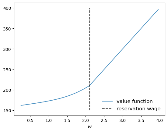
We compute the reservation wage as the first \(w\) such that \(\sigma(w)=1\).
res_wage = w_vals[jnp.searchsorted(σ_star, 1.0)]
fig, ax = plt.subplots()
ax.plot(w_vals, v_star, alpha=0.8, label="value function")
ax.vlines((res_wage,), 150, 400, 'k', ls='--', label="reservation wage")
ax.legend(frameon=False, fontsize=12, loc="lower right")
ax.set_xlabel("$w$", fontsize=12)
plt.show()
9.2. Exercise#
Exercise 9.1
In the setting above, the agent is risk-neutral vis-a-vis future utility risk.
Now solve the same problem but this time assuming that the agent has risk-sensitive preferences, which are a type of nonlinear recursive preferences.
The Bellman equation becomes
When \(\theta < 0\) the agent is risk sensitive.
Solve the model when \(\theta = -0.1\) and compare your result to the risk neutral case.
Try to interpret your result.
Solution to Exercise 9.1
RiskModel = namedtuple('Model', ('n', 'w_vals', 'P', 'β', 'c', 'θ'))

def create_risk_sensitive_js_model(
        n=500,       # wage grid size
        ρ=0.9,       # wage persistence
        ν=0.2,       # wage volatility
        β=0.99,      # discount factor
        c=1.0,       # unemployment compensation
        θ=-0.1       # risk parameter
    ):
    "Creates an instance of the job search model with Markov wages."
    mc = qe.tauchen(n, ρ, ν)
    w_vals, P = jnp.exp(mc.state_values), mc.P
    P = jnp.array(P)
    return RiskModel(n, w_vals, P, β, c, θ)


@jax.jit
def T_rs(v, model):
    """
    The Bellman operator Tv = max{e, c + β R v} with

        e(w) = w / (1-β) and

        (Rv)(w) = (1/θ) ln{E_w[ exp(θ v(W'))]}

    """
    n, w_vals, P, β, c, θ = model
    h = c + (β / θ) * jnp.log(P @ (jnp.exp(θ * v)))
    e = w_vals / (1 - β)

    return jnp.maximum(e, h)


@jax.jit
def get_greedy_rs(v, model):
    " Get a v-greedy policy."
    n, w_vals, P, β, c, θ = model
    e = w_vals / (1 - β)
    h = c + (β / θ) * jnp.log(P @ (jnp.exp(θ * v)))
    σ = jnp.where(e >= h, 1, 0)
    return σ


def vfi(model, max_iter=10_000, tol=1e-4):
    "Solve the infinite-horizon Markov job search model by VFI."
    print("Starting VFI iteration.")
    v = jnp.zeros_like(model.w_vals)    # Initial guess
    i = 0
    error = tol + 1

    while error > tol and i < max_iter:
        new_v = T_rs(v, model)
        error = jnp.max(jnp.abs(new_v - v))
        i += 1
        v = new_v

    v_star = v
    σ_star = get_greedy_rs(v_star, model)
    return v_star, σ_star


model_rs = create_risk_sensitive_js_model()

n, w_vals, P, β, c, θ = model_rs

%time v_star_rs, σ_star_rs = vfi(model_rs)
Starting VFI iteration.
CPU times: user 1.25 s, sys: 376 ms, total: 1.63 s
Wall time: 718 ms
We run it again to eliminate the compilation time.
%time v_star_rs, σ_star_rs = vfi(model_rs)
Starting VFI iteration.
CPU times: user 1.16 s, sys: 381 ms, total: 1.54 s
Wall time: 531 ms
res_wage_rs = w_vals[jnp.searchsorted(σ_star_rs, 1.0)]
fig, ax = plt.subplots()
ax.plot(w_vals, v_star,  alpha=0.8, label="RN $v$")
ax.plot(w_vals, v_star_rs, alpha=0.8, label="RS $v$")
ax.vlines((res_wage,), 150, 400,  ls='--', color='darkblue', alpha=0.5, label=r"RV $\bar w$")
ax.vlines((res_wage_rs,), 150, 400, ls='--', color='orange', alpha=0.5, label=r"RS $\bar w$")
ax.legend(frameon=False, fontsize=12, loc="lower right")
ax.set_xlabel("$w$", fontsize=12)
plt.show()
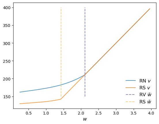
The figure shows that the reservation wage under risk sensitive preferences (RS \(\bar w\)) shifts down.
This makes sense – the agent does not like risk and hence is more inclined to accept the current offer, even when it’s lower.